• 三维散点图
• 脸谱图
• 平行坐标图
• 数据空间的形态
  • 密度
• 均匀程度

加载数据

library(tidyverse)

cjb <- read.csv("/home/wy/Downloads/cjb.csv",
                header = TRUE,
                stringsAsFactors = FALSE,
                fileEncoding = "UTF-8")

三维散点图

plot3d(
  x=cjb$sx,
  y=cjb$wl,
  z=cjb$sw,
  xlab = "Math",
  ylab="Physics",
  zlab = "Biology",
  type = "s",
  size = 0.6,
  col = c("red","green")[cjb$wlfk]
)

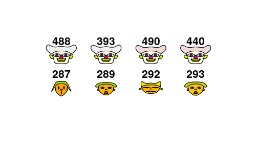
脸谱图

library(aplpack)
select_cols <- c("wl","hx","sw")
select_rows <- c(488,393,490,440,
                 287,289,292,293)
faces(cjb[select_rows,select_cols],
      ncol.plot = 4,
      nrow.plot = 2,
      face.type =1)

effect of variables:
 modified item       Var 
 "height of face   " "wl"
 "width of face    " "hx"
 "structure of face" "sw"
 "height of mouth  " "wl"
 "width of mouth   " "hx"
 "smiling          " "sw"
 "height of eyes   " "wl"
 "width of eyes    " "hx"
 "height of hair   " "sw"
 "width of hair   "  "wl"
 "style of hair   "  "hx"
 "height of nose  "  "sw"
 "width of nose   "  "wl"
 "width of ear    "  "hx"
 "height of ear   "  "sw"

平行坐标图

cjb_top_w <- cjb %>%
  filter(wlfk=="文科") %>%
  mutate(zcj = rowSums(.[4:12])) %>%
  arrange(zcj) %>%
  select(4:13) %>%
  mutate_at(vars(yw:sw),jitter) %>%
  head(n= 50)

cjb_top_l <- cjb %>%
  filter(wlfk=="理科") %>%
  mutate(zcj = rowSums(.[4:12])) %>%
  arrange(zcj) %>%
  select(4:13) %>%
  mutate_at(vars(yw:sw),jitter) %>%
  head(n= 50)

cjb_top <- rbind(cjb_top_w,cjb_top_l)
GGally::ggparcoord(cjb_top,columns =1:9,groupColumn = 10)+
  geom_point()

数据空间的形态

密度

breaks <- c(0,seq(50,100,len=11))
wl_sx_freq <- cjb %>%
  select(wl,sx) %>%
  mutate_at(
    vars(wl,sx),
    function(x){
      cut(x,breaks = breaks)
    }
  )%>%
  group_by(wl,sx) %>%
  summarise(freq = n()) %>%
  complete(wl,sx,fill = list(freq=0))

wl_sx_freq
# A tibble: 1,453 x 3
# Groups:   wl [12]
# wl     sx       freq
# <fct>  <fct>   <dbl>
# 1 (0,50] (0,50]      1
# 2 (0,50] (50,55]     0
# 3 (0,50] (55,60]     0
# 4 (0,50] (60,65]     4
# 5 (0,50] (65,70]     4
# 6 (0,50] (70,75]     2
# 7 (0,50] (75,80]     0
# 8 (0,50] (80,85]     1
# 9 (0,50] (85,90]     0
# 10 (0,50] (90,95]     1
# … with 1,443 more rows

ggplot(wl_sx_freq,aes(x=wl,y=sx,fill=freq))+
  geom_tile(colour="white",size = 0.5)+
  geom_text(aes(label=freq),size=3)+
  scale_fill_gradient(low = "white",high = "red")+
  theme(axis.title.x = element_text(
    angle = 90,
    hjust = 1,
    vjust = 0.5
  ))+
  coord_fixed()

均匀程度

library(clustertend)

set.seed(2012)
scores <- cjb %>%
  select(yw:sw)
n <- floor(nrow(cjb)*0.05)
hopkins_stat <- unlist(replicate(100,hopkins(scores,n)))
mean(hopkins_stat) # [1] 0.09244976