单基因的差异分析
| gene | group | |
|---|---|---|
| TCGA-M9-A5M8-01A-11R-A28J-31 | 2375 | Tumor |
| TCGA-R6-A6DQ-01B-11R-A31P-31 | 4132 | Tumor |
| TCGA-LN-A9FP-01A-31R-A38D-31 | 1447 | Tumor |
| TCGA-LN-A4MQ-01A-11R-A28J-31 | 3247 | Tumor |
| TCGA-JY-A93D-01A-11R-A38D-31 | 1806 | Tumor |
df <- read.csv("expr_mRNA_group.csv",row.names = 1)
boxplot(log2(gene)~group,data=df,col=c("green","red"))
## 计算p
wilcoxTest <- wilcox.test(gene~group,data=df)
pValue <- wilcoxTest$p.value
conGeneMeans <- mean( subset(df,group=="Normal")$gene)
treatGeneMeans <- mean( subset(df,group=="Tumor")$gene)
## 计算logFC
logFC <- log2(treatGeneMeans/conGeneMeans)

图片alt
使用wilcox.test进行统计检验时应该使用那种表达量, FPKM还是count?
单基因的配对差异分析
单基因临床相关性分析

图片alt
KS检验
kruskal.test(expr$YTHDC1~expr$stage)
kruskal.test(YTHDC1~stage,data=expr)
#boxplot(YTHDC1~stage,data=expr)
library(ggplot2)
library(ggpubr)
compare_means(YTHDC1 ~ stage, data = expr,method = "kruskal.test")
my_comparisons <- list( c("Stage I", "Stage II"),c("Stage I", "Stage III"),c("Stage I", "Stage IV"))
expr %>%
  ggplot(aes(x=stage,y=YTHDC1))+
  stat_boxplot(geom="errorbar",width=0.15,aes(color=stage))+
  geom_boxplot(aes(fill=stage),outlier.colour = NA)+
  ylim(5, 8)+
  stat_compare_means(comparisons = my_comparisons)+
  stat_compare_means(method = "kruskal.test",label = "p.format")
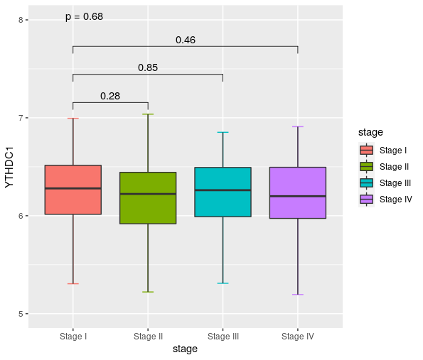
图片alt
逻辑回归
y <- ifelse(expr$YTHDC1>median(expr$YTHDC1),1,0)
logistic <- glm(y~expr$stage,family = binomial(link="logit"))
conf <- confint(logistic,level = 0.95)
summ <- summary(logistic)
cbind(OR=exp(summ$coefficients[,1]),
      OR.95L=exp(conf[,1]),
      OR.95H=exp(conf[,2]),
      p=summ$coefficients[,4])
| OR | OR.95L | OR.95H | p |
|---|---|---|---|
| 1.135135135 | 0.729863084 | 1.772778681 | 0.574001544 |
| 0.813186813 | 0.476284767 | 1.383923034 | 0.446310221 |
| 0.923579109 | 0.525114777 | 1.620832838 | 0.781756194 |
| 0.853422619 | 0.438620318 | 1.656265771 | 0.639262696 |